ISSN: 1839-9940Journal of Genomics

J Genomics 2014; 2:1-19. doi:10.7150/jgen.5054 This volume Cite
Research Paper
Meta-Analysis of Candidate Gene Effects Using Bayesian Parametric and Non-Parametric Approaches
Xiao-Lin Wu1,2 ![]() , Daniel Gianola1,2,3, Guilherme J. M. Rosa2,3, Kent A. Weigel1
, Daniel Gianola1,2,3, Guilherme J. M. Rosa2,3, Kent A. Weigel1
1. Department of Dairy Science, University of Wisconsin, Madison, WI 53706, USA;
2. Department of Animal Sciences, University of Wisconsin, Madison, WI 53706, USA;
3. Department of Biostatistics and Medical Informatics, University of Wisconsin, Madison, WI 53706, USA.
Abstract
Candidate gene (CG) approaches provide a strategy for identification and characterization of major genes underlying complex phenotypes such as production traits and susceptibility to diseases, but the conclusions tend to be inconsistent across individual studies. Meta-analysis approaches can deal with these situations, e.g., by pooling effect-size estimates or combining P values from multiple studies. In this paper, we evaluated the performance of two types of statistical models, parametric and non-parametric, for meta-analysis of CG effects using simulated data. Both models estimated a “central” effect size while taking into account heterogeneity over individual studies. The empirical distribution of study-specific CG effects was multi-modal. The parametric model assumed a normal distribution for the study-specific CG effects whereas the non-parametric model relaxed this assumption by posing a more general distribution with a Dirichlet process prior (DPP). Results indicated that the meta-analysis approaches could reduce false positive or false negative rates by pooling strengths from multiple studies, as compared to individual studies. In addition, the non-parametric, DPP model captured the variation of the “data” better than its parametric counterpart.
Keywords: Bayesian models, candidate genes, Dirichlet process prior, Markov chain Monte Carlo, meta-analysis.
Introduction
Candidate gene (CG) approaches constitute a complementary strategy to map-based cloning and insertional mutagenesis [1-2]. A candidate gene is either a cloned gene presumed to be involved in the regulation and expression of a given trait (“functional candidate”) or a gene closely linked to loci controlling the trait (“positional candidate”). An appealing feature of the CG approach is that it does not require the development of mapping populations, and the analysis relies simply on association tests between polymorphisms of a molecular marker (or markers) and variation for the trait of interest.
Candidate gene approaches have been widely used for identification and characterization of Mendelian and quantitative trait loci (QTLs) in the past decade [3], because they are simple and convenient. The number of published candidate gene studies has been increasing [4]; In pigs, for example, a search in PubMed (http://www.ncbi.nlm.nih.gov/sites/entrez) shows over 40 published papers about candidate genes on litter size, since the work of Rothschild et al. (1996) [2]. This number represents those deposited in the PubMed databases, which makes up only a portion of the studies that have been conducted so far in search for genes affecting pig litter size.
The large number of candidate gene studies, however, does not provide an indication of the reliability of these results, and their conclusions tend to be inconsistent among individual studies. Frequently, when a candidate gene is studied by several groups or even by the same group using different experimental populations, each association found previously can be paired with an equally convincing rebuttal, and both positive and negative findings are likely to be observed in reality. Even when a genuine genetic association exists, the effect size of the gene varies among different studies, hence leading to various conclusions. Such inconsistencies may result from differences in many issues, which include and not limited to varied populations, methodologies, and experimental designs used in CG studies.
This aforementioned situation can be handled by meta-analyses, which typically involves pooling effect-size estimates or combining P values from multiple studies to arrive at an overall conclusion [5,6]. Both fixed-effects and random-effects models have been proposed for meta-analyses [3]. Often, the model poses a center-specific “true effect” while taking into account the heterogeneity over individual studies [7,8]. Hence, meta-analyses provides a powerful tool for assessing population-wide effects of candidate genes on quantitative traits and it can reveal diversity or heterogeneity that are previously undiscovered [9,10].
Current meta-analytic random-effects models assume that the CG effect size among studies is normally distributed, which may not be true in reality. For instance, in a meta-analysis evaluating the association of the platelet PIA polymorphism of glycoprotein IIIa and risk of coronary heart disease, Burr et al. (2003) found that kernel density estimates of study-specific CG effects were multi-modal [7], which obviously violated the normality assumption. In reality, population stratification and admixture is common, leading to multi-modal distributions of the data [11].
In the present paper, we first show how a mixed-effect model can be used to describe the effects of a candidate gene obtained from multiple studies, and then we extend this meta-analytic model to non-parametric settings. The parametric model assumes a normal distribution of study-specific gene effects (referred to as the meta-NP model) whereas the non-parametric model relaxes the normality assumption by replacing it with a more general, discrete, “nonparametric prior” - the Dirichlet process prior (referred to as the DPP model). Both models are implemented within the Bayesian framework. Features of these methods are illustrated using simulated data.
Statistical Methods
Mixed models for study-specific CG effects
Consider N studies that investigate the effect of a candidate gene on a quantitative trait (the methodology can be extended to a set of candidate genes evaluated jointly). Let yi be a point estimate of the effect size ui of the candidate gene (e.g., additive or dominance effects, measured as a linear function of genotypic values) in the i-th study, each representing a single population. Then, yi's can be modeled as:
yi | ui, σi2 ~ N (ui, σi2), for i=1,…,N. (1)
Where σi2 is assumed to be known but empirically equal to the sample variance, si2 in the i-th population. The assumption σi2 = si2 is typically made in meta-analysis, which ensures the parameter identification in the model. This assumption is valid as long as sample sizes in individual studies are not small [7,12].
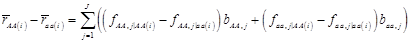
Specifically, if we let yi be the estimated additive effect of the candidate gene in the i-th population, computed as one half of the difference between mean values of the two homozygotes, then, assuming no interactions between this gene and other genes also affecting the trait of interest, we have
(2)
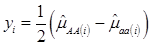
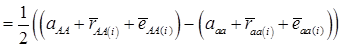
where, for examples,  is an estimate of the genetic effect of genotype AA, pertaining to the i-th study, aAA is its true genetic value,
  is the average residual genetic values of individuals having genotype AA, and
  is the average of the errors for all individuals having genotype AA at the CG locus. The residual genetic values are attributable to loci other than the candidate gene under investigation. The assumption made in (2) is that the candidate gene is the functional gene affecting the trait. If the candidate gene is only a marker linked to a functional gene, its association (additive) effect, denoted as a*, can be expressed as a function of the gene effect a and of the recombination rate r between the marker and the causal gene, e.g., a* = a(1-2r).
Evidently, if  and
and  , then
  provides an unbiased estimator of (aAA - aaa). This situation, however, is unlikely to be true because it rests on over-simplified assumptions. For instance, the genetic determination of a quantitative trait may involve some major genes as well as polygenic effects, and occasional associations between these genes and the quantitative trait can lead to misinterpretation of estimated candidate gene effect, unless they are accounted for properly. Assuming that the quantitative trait is additively affected by J major genes, as well as infinitesimal gene effects, then, without considering interactions among them,
  can be decomposed as:
(3)
where, for example, bAA,j is the effect of genotype AA for the j-th major gene, fAA,j|AA(i) is the frequency that the genotype of the j-th major gene is AA for all individuals whose genotype at the CG locus is also AA, and  is the average value of polygenes of individuals having genotype AA in the i-th population (candidate gene study). Then, if we denote
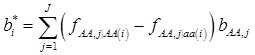
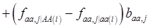 and
and 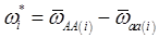 , the first term bi* reflects genetic “noise” due to some major genes affecting the trait, whereas ωi* is attributable to polygenic effects. Thus, it becomes apparent that assuming
  may not be as reasonable as one can expect. In reality,
  due to effects of major genes and polygenes that are not randomized among the three CG genotype groups.
Now, let's revisit (2). Denote aAA-aaa=2μ, which is invariant across individuals populations. Thus, we have:
yi = μ + gi + ei (4)
where  . Here, we assume ei ~ N(0, si2), where si2 is approximated by the variance of the estimate in study i. This decomposition of candidate gene effects suggests that a mixed-effect model can be used to model candidate gene effects estimated from multiple studies. In (4), μ corresponds to the “central” putative effect of the candidate gene, and gi represents random study-specific deviations from the “central” effect size in the i-th study with some variance. Therefore, as long as the genetic background is not randomized properly in a CG study, we have E(gi) ≠ 0 and estimated CG effect in an individual CG study is biased even if this candidate gene represents the true function mutation of the QTL.
In a meta-analysis, however, the estimation of the “central” effects involves weighting estimates from single studies across a variety of genetic backgrounds. This can be viewed as kind of randomization of the genetic background effects across multiple experiments in some sense, which in turn can minimize the bias in estimated CG effects. Re-write (4) in matrix notation as:
(5)
Where y = (y1 y2 … yN)', g = (g1 g2 … gN)', and  is an N×N known (diagonal) covariance matrix with
  being the i-th diagonal element with all off-diagonal elements being equal to zero. Further, we assume that the gi's follow the same normal distribution with mean zero and variance σg2. That is,
(6)
Here, σg2 is the variance of study-specific deviations of the CG effect from the overall mean μ due to background major genes and polygenes.
To complete the Bayesian settings, a normal and a scaled inverse chi-square prior distribution are assumed for μ and σ2, respectively. That is, p(μ) = N (μ0, σμ2) and  , where μ0, σμ2, υg and Ѕg2 are known hyper-parameters.
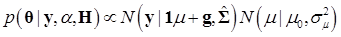
Denote θ = (μ, g, σg2), and let H represents all known hyperparamters. Then, the joint distribution of θ given the data y and hyperparameters H is
(7)
The joint posterior distribution can be evaluated by using a Markov chain Monte Carlo approach such as Gibbs sampling where posterior samples are drawn from the fully conditional distributions of the model parameters, either element-by-element or block-wise [13]. Briefly, the conditional posterior distribution of μ is the normal distribution
(8)
where:
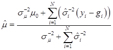
and
In (8), “else” is used to represent all parameters other than μ. The conditional posterior distribution of g is multivariate normal:
(9)
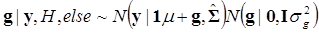
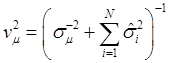
where 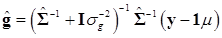 and
and 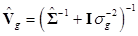 . Finally, the fully conditional distribution of the genetic variance σg2 is the scaled inverse Chi-squared distribution:
(10)
Bayesian non-parametric hierarchical model
There are essentially two normality assumptions in the parametric model. The first one, as seen in (1), relies on the central limit theory. In other words, the sampling distribution of the estimate of a candidate gene effect tends to be a normal distribution as the sample size increases. However, the second normality assumption about the distribution of study-specific CG effects, as in (4), does not have any theoretical justification. For example, Burr et al. (2003) gave evidences of non-normality of CG effects among a number of independent studies [7].
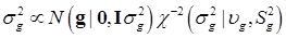
Considering that the candidate gene effect sizes over multiple studies can departure from a homogeneous normal distribution, we replace (6) with  ,
,  , where G is some general distribution, G ~ π, and π is a “nonparametric prior”. A choice for π is the Dirichlet process [14-16]. That is,
G ~ DP(αG0) (11)
Above, G0 is a “baseline” distribution function, which is also referred to as the “center” of the DP prior, in the sense that for any given θ we have E(G(θ)) = G0 (θ), and α is interpretable as a precision parameter indicating the degree of concentration of the prior on G around some parametric family { G0(θ); θ∈Θ}. We assume G0 (σg2) ≡ N (gi |0, σg2), where σg2 is the variance of the baseline distribution G0.
Denote θ ={ μ, g, σg2}, and let H contain all known hyper-parameters. In the first stage, it is assumed that the value of α is known. So, the joint conditional distribution of θ, given y, H, and is
(12)
Above, g ~ G denotes that the gi's follow the unknown distribution G, drawn from a Dirichlet process with G0 ≡ N (gi |0, σg2) as base measure and known precision parameter μ. The notation [gk ~ G][G ~ DP(αG0(μ, σg2))] indicates that the distribution G is integrated out using the DP process as mixing entity. A priori, μ and σg2 follow the same distributions as their counterparts in the parametric model discussed previously.
Bayesian implementation of this meta-DPP model via Markov chain Monte Carlo can be conducted following Gianola et al. (2010) [17] and Wu et al. (2011) [18]. Briefly, given everything else, the posterior distribution of μ in the non-parametric model is normal with the same form as in (8). Since the posterior distribution of μ is not changed when switching to a DP prior, sampling of μ is as in the parametric model. But sampling the gi's in the non-parametric model is different from that in the parametric model. The conditional posterior distribution of gi, given anything else, can be expressed as
(13)
Here, because random distribution G has been integrated out at this point, one does not need to sample G. In (13), we observe that that the fully conditional posterior distribution of gi is a mixture of N-1 degenerate distributions, δ(gi'), with point mass at gi, (i'≠i), and of the parametric conditional distribution under the assumption of a baseline distribution. Specifically, if α→∞, with G0 ≡ N(0, σg2), then (13) tends to (9). In other words, the posterior distribution of g in the non-parametric model is approaching a normal distribution as α→∞.
In essence, the posterior distribution of g is discrete, implying a clustering property of this meta-DPP model. This in turn groups candidate gene effects with similar effects from multiple studies. Let γ1,…, γk, be K distinct values among N estimates of the gene effect size g1,…, gN, where 1≤K≤N, at the t-th iteration of the sampler. Then, the unique values of g1,…, gN induce a partitioning into K clusters. For each cluster, say k, the gj's take on the same value γk. Given that g1,…, gN are random, this induces a random portion as well [17,18]. In the Bayesian context, the marginal posterior distribution of the number of clusters can be constructed, e.g., by directly counting the number of distinct values of gi's at each iteration of the sampler. Following Bush and MacEachern (1996), we re-sample the γ's after the groups of effects are determined, which improves mixing [19].
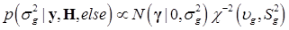
Assuming a scaled inverse chi-square prior distribution, σg2 ~ χ-2(υg,Sg2), the conditional posterior distribution of σg2 is also scaled inverse chi-square:
(14)
Finally, the precision parameter α can be treated as unknown and estimated in the analysis. Following West (1992) [20], given a Gamma prior distribution, p(α) = Gamma(a,b), the fully conditional distribution of α is a mixture of two Gamma distributions, with the mixing probabilities being πs and 1 - πs, as:
(15)
where a* = K + a, b* = b- log s, and 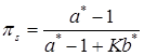 . The auxiliary variable s is drawn from a Beta distribution (Gianola et al., in press):
p(s|K, α, else) = Beta (α+1, K) (16)
Simulation studies
QTL, candidate gene, and the quantitative trait
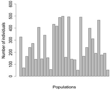
Five meta-analyses were simulated, each consisted of 30 individual studies. In principle, each study represented a specific population under investigation, with the number of individuals per population (sample size) ranging from 52 to 498 (Figure 1). Among them, four populations consisted of less than 100 individuals (i.e., 71, 57, 52, 53 individuals, respectively), mimicking real situations in which samples in large numbers can be difficult to obtain.
Number of individuals per population in the simulation studies.
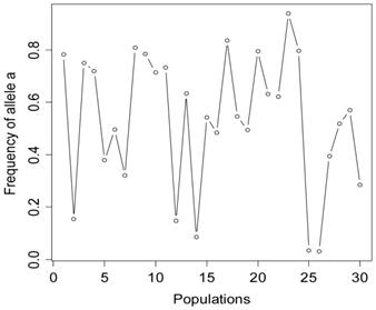
The simulation studies were conducted under two scenarios. The first scenario, as in the first meta-analysis, assumed that the quantitative trait was affected by one bi-allelic QTL and infinitesimal gene effects as well. The additive effect for the QTL was 0.8 units, and the dominance effect of the QTL was non-existent. Essentially, this was an additive QTL. For the sake of simplicity, a bi-allelic candidate gene was simulated, which exactly coincided with the QTL. In other words, the candidate gene fully represents a functional mutation of the QTL. The effect size of the candidate gene alleles followed the order A > a. The allelic frequencies (say allele a) of the candidate gene varied in the 30 populations, ranging from 0.166 to 0.845 (Figure 2). Assuming random mating, instances of the three genotypes at the candidate gene locus were generated from the multinomial distribution
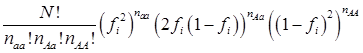
where fi is the frequency of allele a and, for example, naa is the number of individuals having genotypes aa in the i-th population, with N = naa + nAa + nAA.
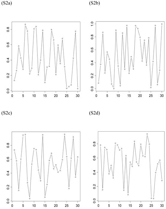
The second scenario was represented by four simulation studies (denoted by S2a, S2b, S2c, and S2d), in which the quantitative trait was genetically determined by two QTLs, one additive and one dominant, and by infinitesimal genetic effects as well. The two QTLs were not linked. The additive effect of both QTLs was 0.6. The dominance effect was 0 for the first QTL and it was 0.3 for the second QTL. Again, the candidate gene fully represented a functional mutation of the first QTL affecting the quantitative trait. The allele frequencies of the first QTL were comparable among populations, which was approximately 0.4 for allele a and 0.6 for allele A, but the allele frequencies of the second QTL varied in the 30 populations, ranging between 0 and 1 (Figure 3). The genotypes of a QTL (candidate gene) were sampled from a multinomial distribution with probability, say, p(G=aa) = fi2, p(G=Aa) = 2fi (1- fi), and p(G=AA) = (1- fi)2, where fi is the frequency of allele q (or a) at the i-th population. Under both scenarios, the overall mean was the only fixed effect, which was arbitrarily given. The infinitesimal genetic effects of each individual followed a normal distribution with mean zero and variance 1.0. The residuals of the phenotypic values followed a normal distribution with mean zero and variance 4.
Frequencies of allele a at the candidate gene locus in 30 populations, as generated in simulation S1.
Frequencies of allele q of the second QTL (not the candidate gene) affecting the trait in the 30 populations, as generated in simulations S2a, S2b, S2c, and S2d. The candidate gene is the first QTL itself, whose allelic frequencies are on average 0.4 for allele a and 0.6 for allele A, respectively.
The quantitative trait for each individual was simulated as the sum of the overall mean, QTL effects, infinitesimal effects, and residuals. Systematic environmental factors were not considered in this series of simulation studies, yet they can be relevant in practical situations. The data used in the subsequent meta-analysis consisted of additive and dominance effects of the candidate gene estimated from a total of 30 populations, which is described as follows. For each population, the additive effect of the candidate gene was computed as:
(17)
where  and
and  were means of the quantitative trait of all individuals having genotype AA and aa, respectively. Assuming homogeneous variance for the three genotypes of the candidate gene, the variance is estimated by:
(18)
where, for example, naa(i) and S2aa(i) are the number of individuals and the sample variance of genotype aa. Then, the standard error of the additive effects is calculated as:
(19)
The dominance effect of the candidate gene and the standard error in the i-th study are computed, respectively, by:
(20)
and
(21)
where  is the trait mean of all individuals having genotype Aa and nAa(i) is the corresponding sample size. In addition, additive and dominance effects of these candidate genes were also estimated using the linear regression approach. Briefly, the genotypes are coded as -0.5 (aa), 0 (Aa), and 0.5 (AA) for the additive effect, and -0.5 (aa), 1 (Aa), and -0.5 (AA) for the dominance effect. Regression coefficients were estimated using the lm function provided by the R Stats package [21].
Markov chain Monte Carlo sampling
The meta analysis was implemented by Bayesian analysis via Markov chain Monte Carlo (MCMC) sampling, based on the meta-NP and the meta-DPP models, respectively. Each analysis consisted of 200,000 iterations after a burn-in period of 2,000 iterations. The posterior samples were thinned every one-tenth and saved for posterior inference of model parameters. Convergences of the chains were diagnosed visually, and all the chains converged and mixed well.
Results and Discussion
Estimation of candidate gene effects in multiple studies
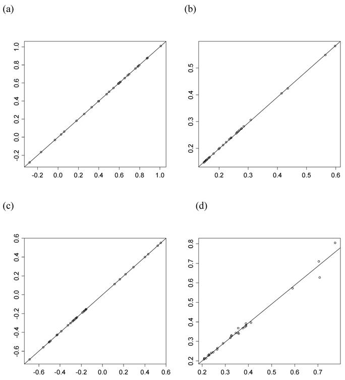
For each of the 30 CG studies, additive and dominance effects (and their standard errors) of the candidate genes were calculated using formula (17)-(21), and presented in Tables 1 and 2, respectively. These estimates corresponded well to those obtained using the linear regression approach. For example, plots of linear fitting between estimated additive and dominance effects of the candidate gene (and their standard errors) obtained using both approaches in meta-analysis S2a are illustrated in Figure 4. The R2, which measures the goodness of fit between estimates obtained using both approaches, was approximately 1 for both additive and dominance effects, and for their standard errors.
Conclusions from individual CG studies varied drastically. In meta-analysis S1, for example, additive effects of the candidate gene varied dramatically among the 30 independent studies, ranging from 0.059 to 1.630 (Table 1). The differences reflected largely the consequence of genetic sampling of the QTL and infinitesimal genes. While most independent studies suggested the presence of significant (p<0.05) or very significant (p<0.001) additive effect of the candidate gene, there were several studies (i.e., from 5 to 10 studies in each of the meta-analysis) showing non-significant (p>0.05) results. In S2d, even negative estimates of additive effect for the candidate gene were obtained in three independent studies, though, by simulation, the additive effect was positive.
The simulated dominance effect of the candidate gene (corresponding to the first QTL) was zero, and estimated dominance effects (Table 2) were not significant (p>0.05) in most of the 30 independent studies. However, as shown in Table 2, there were still five studies supporting the presence of significant dominant effect, with the p values ranging from 0.010 to 0.035.
The above results clearly demonstrated that individual candidate gene studies tend to yield high rates of false positive and false negative results, leading to inconsistent conclusions among individual studies. As was mentioned previously, estimated candidate gene effects are biased if E(gi) ≠ 0, and the bias increases with the difference of allele frequencies of other functional loci affecting the trait. In reality, the bias can result from many factors including linkage and assortative mating, also possibly from population stratification and admixture. In the present simulation studies, genetic sampling of the QTL and infinitesimal gene effect was the major cause of the bias.
Comparison of candidate gene effects and their standard errors obtained using formula (18)-(21) (represented by the y-axis) and those obtained using the linear regression approach (represented by the x-axis) in meta-analysis S2a. These graphs represent: (a) additive effects, (b) standard errors of additive effects, (c) dominance effects, and (d) standard errors of dominance effects.
Mean (standard error) of additive effects of the candidate gene in five meta-analysis studies, each consisting of 30 independent studies 1,2.
| S1 | S2a | S2b | S2c | S2d | |
|---|---|---|---|---|---|
| 1 | 0.773(0.251)** | 0.878(0.182)** | 0.666(0.199)** | 0.320(0.200) | 0.527(0.181)** |
| 2 | 1.111(0.708) | 0.595(0.415) | 0.842(0.393)* | 0.139(0.457) | 0.782(0.401) |
| 3 | 1.151(0.841) | 0.654(0.271)* | 0.689(0.247)** | 0.452(0.292) | 0.464(0.264) |
| 4 | 0.648(0.251)* | 0.181(0.235) | 0.645(0.205)** | 0.823(0.236)** | 0.967(0.232)** |
| 5 | 0.395(0.260) | 0.654(0.214)** | 0.686(0.228)** | 0.169(0.219) | 0.420(0.204)* |
| 6 | 0.059(0.383) | 0.544(0.263)* | 1.256(0.255)** | 0.820(0.273)** | 0.353(0.280) |
| 7 | 0.628(0.194)** | 0.612(0.162)** | 0.704(0.159)** | 0.392(0.168)* | 0.873(0.186)** |
| 8 | 1.630(0.876) | 0.872(0.267)** | 0.778(0.251)** | 0.727(0.275)** | 0.925(0.256)** |
| 9 | 0.695(0.176)** | 0.476(0.199)* | 0.829(0.192)** | 0.473(0.198)* | 0.855(0.188)** |
| 10 | 0.761(0.433) | -0.030(0.309) | 0.069(0.267) | 0.522(0.287) | 0.797(0.278)** |
| 11 | 0.729(0.529) | -0.279(0.598) | 0.374(0.374) | 1.361(0.466)** | 0.388(0.442) |
| 12 | 0.866(0.370)* | 0.786(0.154)** | 0.513(0.152)** | 0.426(0.158)** | 0.306(0.159) |
| 13 | 0.894(0.194)** | 0.760(0.168)** | 0.658(0.163)** | 0.525(0.172)** | 0.546(0.170)** |
| 14 | 0.705(0.192)** | 0.502(0.149)** | 0.618(0.159)** | 0.581(0.137)** | 0.501(0.151)** |
| 15 | 1.182(0.151)** | 0.685(0.152)** | 0.612(0.147)** | 0.533(0.158)** | 0.669(0.156)** |
| 16 | 1.078(0.401)** | 0.256(0.259) | 0.688(0.320)* | 0.548(0.260)* | 0.798(0.262)** |
| 17 | 0.649(0.162)** | 0.606(0.148)** | 0.432(0.150)** | 0.672(0.158)** | 0.830(0.157)** |
| 18 | 0.663(0.314)* | 0.031(0.277) | 1.016(0.294)** | 0.752(0.245)** | 0.973(0.267)** |
| 19 | 0.807(0.496) | 1.009(0.277)** | 0.554(0.272)* | 0.904(0.261)** | 0.050(0.286) |
| 20 | 0.366(0.446) | -0.165(0.565) | 0.485(0.471) | 0.301(0.575) | 1.259(0.413)** |
| 21 | 1.010(0.148)** | 0.399(0.165)* | 0.649(0.158)** | 0.655(0.160)** | 0.354(0.145)* |
| 22 | 1.312(0.233)** | 0.061(0.285) | 0.571(0.280)* | 0.827(0.327)* | 0.141(0.326) |
| 23 | 1.191(0.367)** | 0.783(0.225)** | 0.463(0.236) | 0.459(0.219)* | 0.559**(0.218) |
| 24 | 1.276(0.451)** | 0.684(0.158)** | 0.568(0.164)** | 0.634(0.162)** | 0.348(0.197) |
| 25 | 0.414(0.191)* | 0.697(0.202)** | 0.460(0.207)* | 0.459(0.193)* | 0.811(0.182)** |
| 26 | 0.642(0.239)** | 0.398(0.240) | 0.138(0.242) | 0.708(0.242)** | 0.507(0.249)* |
| 27 | 1.026(0.248)** | 0.591(0.157)** | 0.735(0.161)** | 0.532(0.162)** | 0.617(0.166)** |
| 28 | 1.212(0.288)** | 0.593(0.242)* | 0.493(0.227)* | 0.754(0.268)** | 0.850(0.239)** |
| 29 | 0.906(0.298)** | 0.331(0.262) | 0.975(0.252)** | 0.687(0.230)** | 0.669(0.230)** |
| 30 | 0.282(0.541) | 0.797(0.436) | 1.034(0.495)* | 0.413(0.574) | 0.251(0.413) |
1 S1-S2d = # of meta-analysis studies; 2 1~30 = # of individual studies per meta-analysis study; * p<0.05; ** p<0.01.
Mean (standard deviation) of dominance effect of the candidate gene in five meta-analysis studies, each consisting of 30 individual studies 1.
| S1 | S2a | S2b | S2c | S2d | |
|---|---|---|---|---|---|
| 1 | 0.283(0.314) | 0.113(0.248) | 0.031(0.273) | -0.438(0.270) | -0.002(0.261) |
| 2 | -1.912(0.828)* | -0.153(0.591) | 0.049(0.574) | -0.018(0.587) | 0.348(0.606) |
| 3 | 0.089(0.906) | -0.255(0.376) | 0.520(0.378) | -0.357(0.387) | -0.003(0.381) |
| 4 | -0.194(0.334) | -0.490(0.326) | 0.135(0.294) | 0.128(0.317) | -0.080(0.318) |
| 5 | 0.003(0.352) | -0.325(0.291) | -0.046(0.300) | -0.230(0.306) | -0.308(0.283) |
| 6 | -0.626(0.494) | 0.431(0.383) | -0.035(0.387) | -0.348(0.381) | 0.066(0.399) |
| 7 | -0.142(0.254) | -0.155(0.239) | -0.245(0.226) | 0.181(0.235) | 0.277(0.246) |
| 8 | -1.068(0.954) | 0.521(0.355) | 0.092(0.354) | -0.276(0.383) | -0.012(0.387) |
| 9 | -0.378(0.238) | -0.301(0.265) | -0.089(0.262) | 0.143(0.258) | -0.354(0.270) |
| 10 | 0.043(0.539) | -0.177(0.411) | -0.271(0.368) | 0.489(0.375) | 0.273(0.401) |
| 11 | -0.707(0.656) | -0.171(0.774) | 0.036(0.526) | -0.267(0.623) | 0.157(0.558) |
| 12 | 0.179(0.429) | 0.551(0.229)* | -0.071(0.216) | 0.049(0.220) | -0.228(0.218) |
| 13 | 0.114(0.254) | -0.246(0.225) | -0.121(0.222) | 0.055(0.235) | -0.023(0.234) |
| 14 | 0.017(0.244) | -0.273(0.207) | -0.218(0.221) | -0.088(0.196) | -0.465(0.211)* |
| 15 | 0.368(0.208) | 0.401(0.210) | 0.189(0.209) | -0.028(0.217) | -0.074(0.217) |
| 16 | 0.775(0.511) | -0.282(0.358) | 0.333(0.406) | 0.639(0.365) | 0.220(0.355) |
| 17 | 0.321(0.219) | -0.189(0.209) | 0.009(0.208) | -0.173(0.214) | 0.188(0.213) |
| 18 | 0.213(0.420) | -0.431(0.389) | 0.413(0.397) | 0.132(0.351) | 0.042(0.362) |
| 19 | 0.046(0.593) | -0.687(0.389) | -0.275(0.407) | -0.573(0.357) | -0.749(0.412) |
| 20 | -0.866(0.692) | -0.504(0.704) | -0.621(0.690) | -0.708(0.719) | 0.897(0.626) |
| 21 | 0.260(0.206) | -0.388(0.226) | -0.200(0.215) | 0.004(0.220) | -0.068(0.208) |
| 22 | -0.267(0.333) | 0.219(0.389) | 0.149(0.394) | -0.254(0.413) | -0.397(0.409) |
| 23 | -0.008(0.450) | -0.265(0.321) | -0.197(0.318) | 0.127(0.309) | -0.129(0.305) |
| 24 | -0.682(0.489) | -0.500(0.230)* | -0.010(0.233) | 0.271(0.219) | -0.074(0.259) |
| 25 | -0.136(0.270) | -0.160(0.264) | 0.115(0.269) | -0.106(0.279) | 0.168(0.260) |
| 26 | -0.197(0.330) | -0.242(0.326) | 0.001(0.343) | -0.739(0.348)* | 0.217(0.349) |
| 27 | -0.272(0.298) | 0.293(0.217) | 0.201(0.223) | 0.214(0.226) | -0.038(0.232) |
| 28 | -0.423(0.380) | -0.425(0.345) | -0.612(0.332) | -0.162(0.370) | 0.123(0.335) |
| 29 | -0.024(0.402) | 0.165(0.356) | -0.131(0.328) | -0.087(0.331) | 0.162(0.320) |
| 30 | 0.253(0.738) | -0.558(0.708) | 0.557(0.648) | -0.185(0.770) | 0.118(0.627) |
1 S1-S2d = # of meta-analysis studies; 2 1~30 = # of individual studies per meta-analysis study; * p<0.05.
Bayesian parametric meta-analysis of candidate gene effects
In the meta-NP model, in which a normal prior distribution was assumed for the study-specific CG effect, the overall mean estimated the “central” candidate gene effect and it corresponded well to the simulated value of the candidate gene. The overall mean of additive effect of the candidate gene was estimated to be 0.811 in meta-analysis S1 and it was from 0.540 to 0.631 in meta-analyses S2a, S2b, S2c and S2d (Table 3). These estimates agreed with the simulated values of the candidate gene, which were 0.8 in S1 and 0.6 in S2a-S2d, respectively. The 95% highest posterior density (HPD) interval of the additive effects obtained from the meta-NP model always contained the “true” values. Estimated overall mean of dominance effect of the candidate gene was small (for instance, -0.092 in S1 and from -0.124 to -0.021 in S2a-S2d) and not significant because the 95% HPD intervals contained zero (Table 4).
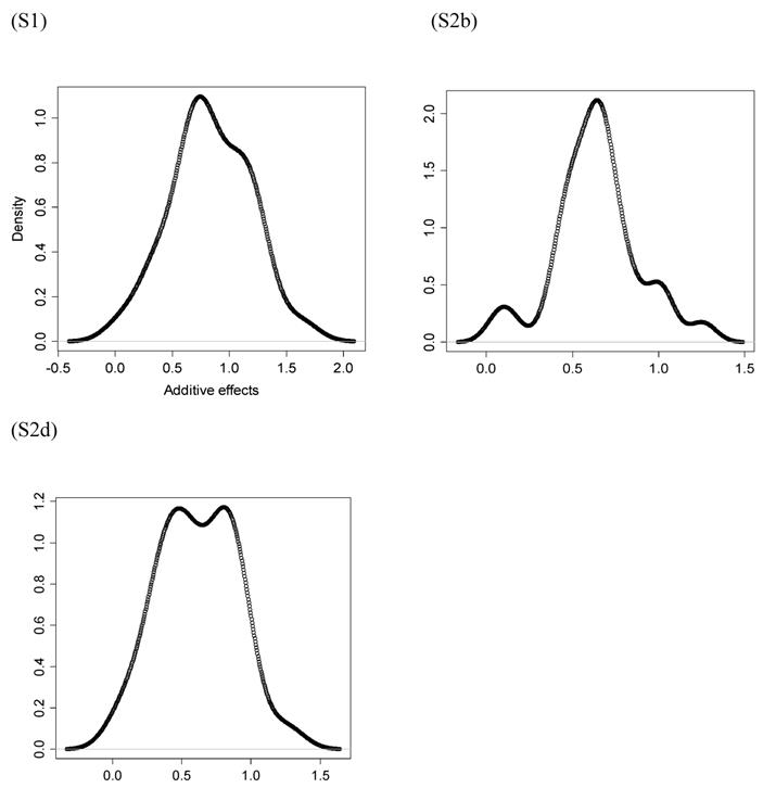
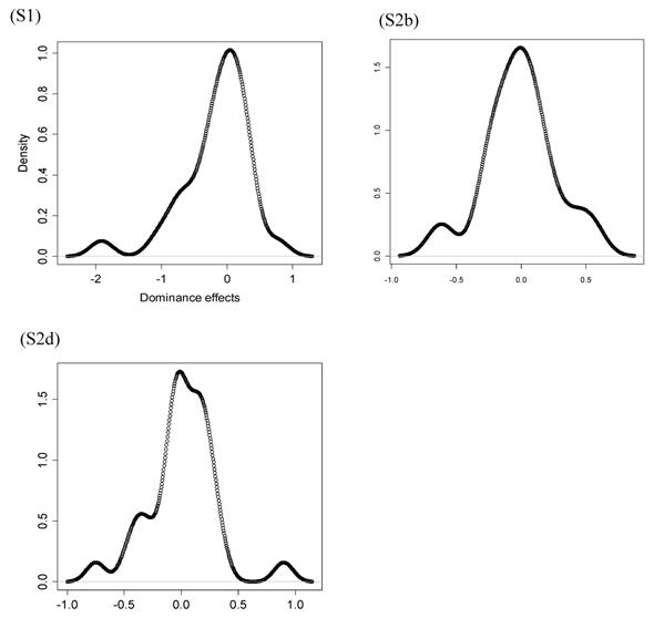
However, the normality assumption for the study-specific deviations of the candidate gene effects is questionable. As shown in Figures 5 and 6, kernel density plots of additive and dominance effects of the candidate gene (e.g., in simulations S1, S2b, and S2d) were multi-modal, and them by no means looked like “bell-shaped” normal distributions. This finding coincided with that of Bur et al (2003) [7].
Bayesian non-parametric meta-analysis of candidate gene effects
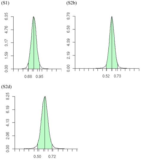
The meta-DPP model relaxed the normality assumption for study-specific CG effect by replacing it with a general prior distribution - the DP prior. Noticeably, the meta-DPP model produced estimates of the “central” candidate gene effects that were generally closer to the simulation values and with smaller standard errors (Table 3), as compared to the parametric method with a normal prior (referred to as the meta-NP method). In S2a, for example, the estimate (standard error) for the mean of the additive effect of the candidate gene was 0.569 (0.058) from the meta-DPP method and 0.540 (0.074) from the meta-NP method. Same patterns were observed in simulations S2b, S2c, and S2d (Table 3). Nevertheless, the overall means of the additive effect from both approaches were similar to each other and they both corresponded well to the “true” value. This high agreement between the two models was probably because the candidate gene was the only major gene (QTL) affecting the quantitative trait in S1, and the effect of genetic sampling was not as dramatic as it was in simulations S2a-S2d when a second QTL was also acting. Even in the latter case, the DPP estimates still had a smaller standard error than the meta-NP estimate. In all five simulations, the 95%HPD interval for the additive effect contained the true values. The posterior distributions of the “central” additive effects were approximately, normally distributed and symmetric, and examples from meta-analyses S1, S2a, and S2c are illustrated in Figure 7.
Summary posterior statistics of additive effects of the candidate gene obtained from the meta-NP and meta-DPP methods 1.
| Simulation2 | Parameter3 | Mean | Median | StdDev4 | 95%HPD5 |
|---|---|---|---|---|---|
| ------ Meta-NP method ------ | |||||
| S1 | μ | 0.811 | 0.810 | 0.086 | 0.643-0.980 |
| σg2 | 0.092 | 0.087 | 0.030 | 0.048-0.165 | |
| S2a | μ | 0.540 | 0.540 | 0.074 | 0.396-0.686 |
| σg2 | 0.075 | 0.075 | 0.025 | 0.039-0.134 | |
| S2b | μ | 0.631 | 0.631 | 0.062 | 0.510-0.752 |
| σg2 | 0.053 | 0.051 | 0.017 | 0.028-0.093 | |
| S2c | μ | 0.577 | 0.577 | 0.061 | 0.457-0.696 |
| σg2 | 0.049 | 0.047 | 0.016 | 0.027-0.087 | |
| S2d | μ | 0.613 | 0.613 | 0.067 | 0.481-0.743 |
| σg2 | 0.064 | 0.062 | 0.020 | 0.034-0.113 | |
| ------ Meta-DPP method ------ | |||||
| S1 | μ | 0.814 | 0.813 | 0.070 | 0.681-0.953 |
| σg2 | 0.690 | 0.630 | 0.280 | 0.294-1.251 | |
| S2a | μ | 0.569 | 0.571 | 0.058 | 0.452-0.680 |
| σg2 | 0.727 | 0.661 | 0.308 | 0.293-1.331 | |
| S2b | μ | 0.625 | 0.625 | 0.055 | 0.522-0.732 |
| σg2 | 0.734 | 0.667 | 0.307 | 0.294-1.334 | |
| S2c | μ | 0.568 | 0.568 | 0.054 | 0.466-0.673 |
| σg2 | 0.739 | 0.672 | 0.310 | 0.300-1.349 | |
| S2d | μ | 0.607 | 0.607 | 0.056 | 0.500-0.718 |
| σg2 | 0.714 | 0.651 | 0.295 | 0.286-1.297 |
1 Meta-NP model = model assuming a normal prior distribution for σg2; Meta-DPP model = model assuming a DPP distribution for σg2;
2 S1-S2d = # of simulation studies.
3 μ = “central” additive effect; σg2 = variance of study-specific deviations of additive effects.
4 StdDev = standard deviation.
5 95%HPD = 95 highest posterior density interval.
Summary posterior statistics of dominance effects of the candidate gene obtained from the meta-NP and meta-DPP models 1.
| Simulation2 | Parameter3 | Mean | Median | StdDev4 | 95%HPD5 |
|---|---|---|---|---|---|
| ------ Meta-NP model ------ | |||||
| S1 | μ | -0.092 | -0.092 | 0.121 | -0.329-0.142 |
| σg2 | 0.164 | 0.154 | 0.059 | 0.079-0.304 | |
| S2a | μ | -0.124 | -0.125 | 0.085 | -0.292-0.041 |
| σg2 | 0.095 | 0.090 | 0.031 | 0.050-0.171 | |
| S2b | μ | -0.021 | -0.022 | 0.076 | -0.167-0.128 |
| σg2 | 0.062 | 0.059 | 0.020 | 0.032-0.114 | |
| S2c | μ | -0.050 | -0.050 | 0.082 | -0.210-0.112 |
| σg2 | 0.079 | 0.075 | 0.026 | 0.040-0.141 | |
| S2d | μ | -0.030 | -0.030 | 0.081 | -0.188-0.127 |
| σg2 | 0.071 | 0.067 | 0.023 | 0.037-0.128 | |
| ------ Meta-DPP model ------ | |||||
| S1 | μ | -0.037 | -0.035 | 0.083 | -0.212-0.120 |
| σg2 | 0.709 | 0.647 | 0.292 | 0.281-1.268 | |
| S2a | μ | -0.118 | -0.119 | 0.079 | -0.267-0.041 |
| σg2 | 0.676 | 0.620 | 0.266 | 0.283-1.197 | |
| S2b | μ | -0.028 | -0.027 | 0.065 | -0.156-0.099 |
| σg2 | 0.735 | 0.666 | 0.309 | 0.282-1.328 | |
| S2c | μ | -0.032 | -0.031 | 0.068 | -0.165-0.096 |
| σg2 | 0.734 | 0.662 | 0.313 | 0.293-1.341 | |
| S2d | μ | -0.044 | -0.044 | 0.067 | -0.174-0.087 |
| σg2 | 0.731 | 0.664 | 0.309 | 0.290-1.313 |
1 Meta-NP model = model assuming a normal prior distribution for σg2; Meta-DPP model = model assuming a DPP distribution for σg2;
2 S1-S2d = # of simulation studies.
3 μ = “central” additive effect; σg2 = variance of study-specific deviations of additive effects.
4 StdDev = standard deviation.
5 95%HPD = 95 highest posterior density interval.
Kernel density plots of additive effects of the candidate gene obtained from 30 independent studies in meta-analyses S1, S2b, and S2d. The X-axis represents additive effect and the Y-axis represents kernel density estimates.
Kernel density plots of dominance effects of the candidate gene obtained from 30 independent studies in simulations S1, S2b, and S2d. The X-axis represents dominance effect and the Y-axis represents kernel density estimates.
Posterior distributions of “central” additive effect of the candidate gene in simulations S1, S2b, S2d, each representing a meta-analysis with 30 individual studies (i.e., 30 independent populations). The x-axis represents values of posterior draws and the y-axis represents kernel density estimates.
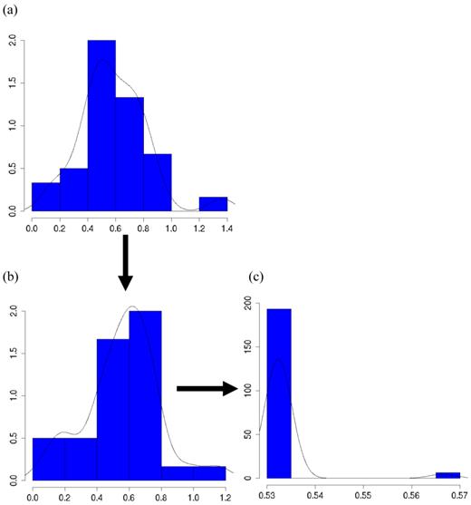
The meta-DPP model captured the feature of the data well because it relaxed the normal assumption about the distribution of the candidate gene effects. In Figure 8a, the histogram and kernel density plots of the estimated additive effects from 30 individual studies in meta-analysis S2c clearly shows a multi-modal distribution, rather than a normal distribution typically assumed in the meta-NP model. Figure 8b shows an instance of initial states of cluster values of study-specific effects (specifically, study-specific effects plus the “central” additive effect μ, such that they are on the same scale as the estimates from the individuals studies), and Figure 8c shows an instance of cluster values during MCMC sampling (the “central” additive effect μ was also added for the sake of comparison). Apparently, the clustering property of the meta-DPP method induced an aggregated structure of the effect sizes of the candidate gene from single studies, which could capture the variation of candidate gene effects obtained from multiple studies.
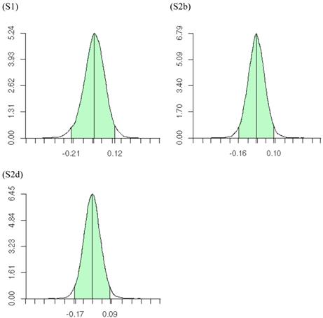
The meta-DPP approach suggested that the dominance effect of the candidate gene was not significant, because the 95% HPD interval contained zero (Figure 9). This was in agreement with the meta-NP approach. Both types of meta-analyses could reduce substantially the chance of reporting false positive or false negative candidate effects on the quantitative trait, as compared to individual candidate gene studies.
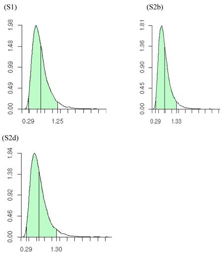
Posterior distributions of the variance of the study-specific CG effects (σg2), as obtained from the meta-DPP method, are illustrated in Figure 10. The estimates (standard deviations) of σg2 obtained from the meta-DPP method were larger than those from the meta-NP method (Tables 3 and 4).
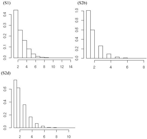
Summary posterior statistics of other model parameters (i.e., K, α, s) are listed in Table 5. On average, the meta-DPP approach postulated from 1.6 to 3.0 clusters for the additive effect, and from 1.7 to 3.5 clusters for the dominance effects in the five simulation studies. The posterior distributions of the number of clusters, e.g., for additive effects of the candidate gene in meta-analysis S1, S2b and S2d, were shown in Figure 11. The posterior means of α were small, ranging from 0.705 to 1.026 for the additive effect and from 0.739 to 1.139 for the dominance effect. This was indication that the data were diffuse, and the distribution of candidate gene effects among studies deviated from a normal distribution. The small values of α might explain the difference in the estimates of σg2 between the two the parametric and non-parametric models. As α becomes large, the distribution of σg2 in the meta-DPP model would approach a normal distribution, and the estimates of σg2 would become comparable between the two approaches.
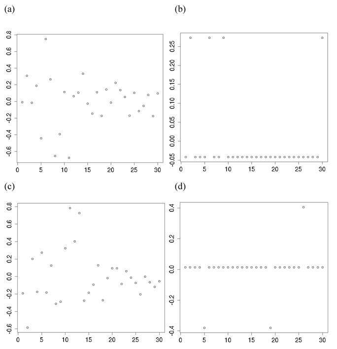
Finally, the clustering of gi's by their inferred values is a noting feature of the non-parametric method with DP prior. In meta-analysis S2b, for example, when the additive effects were initialized as belonging to over 10 clusters, they could converge to two clusters (Figure 12a,b). Similarly, when the dominance effects (e.g., in simulation S2d) were initialized with over 10 clusters, they could converge to approximately three clusters or less (Figure 12c,d). Theoretically, the meta-DPP model can be considered as an infinite model, that is, a mixture model with a countably infinite number of clusters. In practice, however, the probability of drawing gi is decreased quickly, and only a small number of clusters are possibly. Intuitively, imaging we generate samples from  . Because G ~ DP(αG0) is discrete with positive probability, there will be ties among the gi's. So, the gi's will form clumps. When α is small, the first few probabilities Pi's add up to nearly 1, resulting in higher probability ties. This leads to important consequences regarding the posterior distribution of g given the data y. Consider, for example, the distribution of gi. Conditional on the data and g-i (i.e., g without gi), the estimation results in shrinkage towards
  and towards a grand mean. Because of the propensity of clumping, the posterior is also shrunk towards those in g-i whose values are close to
  . This property results in a way of pooling information that involves weighing results of similar studies more heavily [22].
In summary, we have presented and compared two meta-analysis models that were used to evaluate candidate gene effects using simulation data. While both models applied well in the meta-analysis of candidate gene studies, the non-parametric model with DPP captured better the distribution of the candidate gene effects among studies, hence leading to more robust conclusions. The non-parametric model with DPP makes weaker assumption about the distribution of candidate genes among individual studies, and hence it model can outperform the parametric model in fitting the data with cryptic gene interaction. Finally, it should be noted that a candidate gene may not be the causative locus itself, but linked gene. To further identifying causative loci is beyond the scope of the present study. Also, with two QTLs, we did not evaluation their interactions in the present study. Instead, we retain simple QTL settings to compare the performance of the two meta-analysis models.
Summary (posterior) statistics of other model parameters obtained from the meta-DPP model.
| Simulation1 | Parameter2 | Mean | Median | StdDev3 | 95%HPD4 |
|---|---|---|---|---|---|
| ---- Additive effect --- | |||||
| S1 | K | 2.970 | 3.000 | 1.501 | 1.000-6.000 |
| α | 1.026 | 0.906 | 0.613 | 0.112-2.241 | |
| s | 0.063 | 0.055 | 0.042 | 0.008-0.168 | |
| S2a | K | 2.055 | 2.000 | 1.181 | 1.000-4.000 |
| α | 0.817 | 0.707 | 0.513 | 0.067-1.811 | |
| s | 0.057 | 0.048 | 0.040 | 0.006-0.158 | |
| S2b | K | 1.790 | 1.000 | 1.009 | 1.000-4.000 |
| α | 0.753 | 0.652 | 0.468 | 0.064-1.666 | |
| s | 0.055 | 0.046 | 0.040 | 0.006-0.156 | |
| S2c | K | 1.569 | 1.000 | 0.849 | 1.000-3.000 |
| α | 0.705 | 0.613 | 0.444 | 0.052-1.554 | |
| s | 0.054 | 0.045 | 0.039 | 0.005-0.154 | |
| S2d | K | 2.171 | 2.000 | 1.256 | 1.000-5.000 |
| α | 0.840 | 0.726 | 0.522 | 0.058-1.851 | |
| s | 0.058 | 0.049 | 0.041 | 0.006-0.159 | |
| ---- Dominance effect --- | |||||
| S1 | K | 2.658 | 2.000 | 1.549 | 1.000-6.000 |
| α | 0.956 | 0.823 | 0.604 | 0.075-2.140 | |
| s | 0.061 | 0.053 | 0.041 | 0.007-0.162 | |
| S2a | K | 3.452 | 3.000 | 1.540 | 1.000-6.000 |
| α | 1.139 | 1.019 | 0.638 | 0.132-2.398 | |
| s | 0.067 | 0.058 | 0.044 | 0.009-0.173 | |
| S2b | K | 1.716 | 1.000 | 0.982 | 1.000-4.000 |
| α | 0.739 | 0.639 | 0.466 | 0.057-1.638 | |
| s | 0.055 | 0.046 | 0.040 | 0.006-0.155 | |
| S2c | K | 1.945 | 2.000 | 1.134 | 1.000-4.000 |
| α | 0.790 | 0.684 | 0.493 | 0.056-1.758 | |
| s | 0.057 | 0.047 | 0.041 | 0.006-0.160 | |
| S2d | K | 1.878 | 2.000 | 1.103 | 1.000-4.000 |
| α | 0.775 | 0.671 | 0.487 | 0.057-1.707 |
1 S1-S2d = # of simulation studies.
2 K = number of clusters; α = precision parameter; s = auxiliary variable.
3 StdDev = standard deviation.
4 95%HPD = 95 highest posterior density interval.
Histograms and kernel density plots of: (a) additive effects of the candidate gene obtained from 30 studies, (b) initial state of the cluster values, and (c) a state of the cluster values during the MCMC sampling, in simulation S2c.
Posterior distributions of “central” dominance effect of the candidate gene in meta analyses S1, S2b, and S2d, respectively, each consisting of 30 independent studies. The x-axis represents values of posterior draws and the y-axis represents kernel density estimates.
Posterior distributions of the variance of study-specific candidate gene (additive) effects in meta analyses S1, S2b, and S2d, respectively, each consisting of 30 independent studies. The x-axis represents values of posterior draws and the y-axis represents kernel density estimates.
Posterior distributions of the number of clusters of additive effects of the candidate gene in meta analyses S1, S2b, and S2d, respectively, each consisting of 30 independent studies. The x-axis represents values of posterior draws and the y-axis represents kernel density estimates.
Comparison of states of cluster values assigned to the 30 population at the initial stage (left) and a stage after convergence (right), respectively. Graphs (a)-(b) correspond to the model with additive effect in meta-analysis S2b; graphs (c)-(d) correspond to the model with dominance effects in meta-analysis S2d.
Acknowledgements
This research is supported by the Wisconsin Agriculture Experiment Station, and by grant NSF DMS-044371.
Competing Interests
The authors have declared that no competing interest exists.
References
1. Pflieger S, Lefebvre V, Causse M. The candidate gene approach in plant genetics: A review. Mol Breed. 1996;7:275-91
2. Rothschild M, Jacobson C, Vaske D. et al. The estrogen receptor locus is associated with a major gene influencing litter size in pigs. Proc Natl Acad Sci U S A. 1996;93:201-5
3. Wu XL, Hu ZL. Meta-analysis of QTL Mapping Experiments. Methods Mol Biol. 2012;871:145-71
4. Munafò MR. Candidate gene studies in the 21st century: meta-analysis, mediation, moderation. Genes Brain Behav. 2006;5(Suppl 1):3-8
5. DerSimonian R, Laird N. Meta-analysis in clinic trials. Control Clin Trials. 1986;7:177-88
6. Normand ST. Meta-analysis: formulating, evaluating, combining, and reporting. Stat Med. 1999;18:321-59
7. Burr D, Doss H, Cooke GE. et al. A meta-analysis of studies on the association of the platelet PlA polymorphism of glycoprotein IIIa and risk of coronary heart disease. Stat Med. 2003;22:1741-60
8. Burr D. Doss H. A Bayesian semiparametric model for random-effects meta analysis. J Amer Stat Assoc. 2005;100:242-51
9. Ioannidis JP, Ntzani EE, Trikalinos TA. et al. Replication validity of genetic association studies. Nat Genet. 2001;29:306-9
10. Ioannidis JP, Trikalinos TA, Ntzani EE. et al. Genetic associations in large versus small studies: an empirical assessment. Lancet. 2003;361:567-71
11. Clayton D. Population association. In: (ed.) Balding D J, Bishop M, Cannings C. Handbook of Statistical Genetics. Chichester: John Wiley & Sons Ltd. 2001:519-40
12. DuMouchel W. Bayesian meta analysis. In: (ed.) Berry D. Statistical Methodology in the Pharmaceutical Science. New York: Marcel Dekker. 1990:509-29
13. Sorensen D, Gianola D. Likelihood, Bayesian, and MCMC Methods in Quantitative Genetics. New York: Springer-Verlag. 2002
14. Ferguson TS. A Bayesian analysis of some nonparametric problems. Ann Stat. 1973;1:209-30
15. Ferguson TS. Prior distributions on spaces of probability measures. Ann Stat. 1974;2:615-29
16. Antoniak C. Mixtures of Dirichlet process with applications to Bayesian nonparametric problems. Ann Stat. 1974;2:1152-74
17. Gianola D, Wu XL, Manfredi E. et al. A non-parametric mixture model for genome-enabled prediction of genetic value for a quantitative trait. Genetica. 2010;138:959-77
18. Wu XL, Gianola D, Hu ZL. et al. Meta-Analysis of Quantitative Trait Association and Mapping Studies using Parametric and Non-Parametric Models. J Biomet Biostat. 2011 S1
19. Bush CA, MacEachern SN. A semiparametric Bayesian model for randomized block designs. Biometrika. 1996;83:275-85
20. West M. Hyperparameter estimation in Dirichlet process mixture models. Duke University Technical Report 92-A03. 1992
21. R: A language and environment for statistical computing. R Development Core Team. http://www.R-project.org/
22. Escobar MD, West M. Bayesian density estimation and inference using mixtures. J Amer Stat Assoc. 1995;90:577-88
Author contact
![]() Corresponding author: Xiao-Lin Wu, 1675 Observatory Dr., Department of Dairy Science, University of Wisconsin, Madison, WI 53706, USA. Tel.: (608) 263 7824; Fax: (608) 263-9412; E-mail: nick.wuwisc.edu.
Corresponding author: Xiao-Lin Wu, 1675 Observatory Dr., Department of Dairy Science, University of Wisconsin, Madison, WI 53706, USA. Tel.: (608) 263 7824; Fax: (608) 263-9412; E-mail: nick.wuwisc.edu.
Published 2014-1-2